The project had funding for one zoom layer. Each zoom layer requires additional storage.
1. Select the start and end times using the calendar and clock icons.

2. Select the load icon and wait until the data has been loaded. A green message will appear

3. Select the far right icon in the “Animation Control” box that looks like a target.

4. Wait for the entire animation to play through and then select the “Download video” icon.

The video download location is dependent on your computer settings. There have been instances reported where the video will appear to be downloading and then nothing happens. These instances have self-corrected prior to being able to effectively troubleshoot the issue.
This may have occurred from changing the date/time and not loading the data again. The “load” button needs to be selected whenever the time period is modified. It is helpful to refresh the screen and load the data again if the previous reason did not pertain to your problem. If it is close to daylight savings, then a configuration change might be needed.
A gray link means that this segment of freeway was not receiving any speed data during that time period.
No, this feature has not been added. You can change the time period to match the desired duration to the nearest hour. Videos can be trimmed using software outside this tool.
The video will need to be converted to file type compatible to PowerPoint. There are online converter tools for .avi to .wmv files.
A time period was selected outside the data storage available for this graph. The data storage currently has back until May 2015. (Checked 5/25/16)
Computer settings need to be updated to allow .avi media to be viewed with your program.
The freeway was broken into one mile segments. Each segment was categorized as fast or slow if the median speed for the time period was below 50 mph. This threshold speed was chosen because it is the approximate speed to optimize vehicle throughput. A segment was categorized as reliable or unreliable using the buffer time index (BTI) of 0.6. A value of 0.6 means a person will need to add 60% more time to their average travel time to arrive on time 95% of their driving experiences. The greater the BTI value, the more variance in a travel time from day-to-day and thus more unreliable.

Reliability

A vehicle-hour is an additional hour a vehicle had to wait in traffic. It represents lost time from congestion. If the occupancy rate of vehicles was always known then it could be converted to person-hours or an hour a person was delayed.
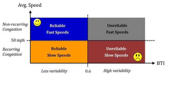
Congestion is identified as any 5 minute interval under 50 mph at each mainline station. The source is determined by looking at internal weather, incident, construction, and traffic speed databases. If indicators for multiple sources are present then a hierarchy of congestion sources is used as shown in the figure below.

Hierarchy of congestion sources

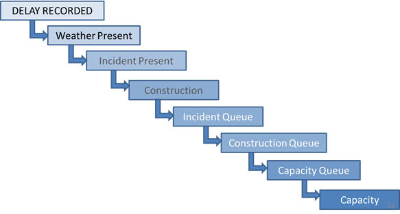
The result of using this approach means that topics near the top of the order exceed the actual amount in delay while those on the bottom are under. Incidents is only the source of congestion while the incident is active. So if an incident is cleared and a long queue still remains then this will be counted as capacity if no other factors are present. This can cause recording less delay than actual caused by incidents.
The 85% and 15% profiles refer to the number of vehicles whose speeds fall below the point indicated on the graph. So, for example, 100% would mean the maximum speeds observed.

AM is 7 am to 8 am, PM is 5 pm to 6 pm.